Let’s build an MP3-decoder!
Even though MP3 is probably the single most well known file format and codec on Earth, it’s not very well understood by most programmers – for many encoders/decoders is in the class of software “other people” write, like standard libraries or operating system kernels. This article will attempt to demystify the decoder, with short top-down primers on signal processing and information theory when necessary. Additionally, a small but not full-featured decoder will be written (in Haskell), suited to play around with.
The focus on this article is on concepts and the design choices the MPEG team made when they designed the codec – not on uninteresting implementation details or heavy theory. Some parts of a decoder are quite arcane and are better understood by reading the specification, a good book on signal processing, or the many papers on MP3 (see references at the end).
A note on the code: The decoder accompanying this article is written for readability, not speed. Additionally, some unusual features have been left out. The end result is a decoder that is inefficient and not standards compliant, but with hopefully readable code. You can grab the source here: mp3decoder-0.0.1.tar.gz. Scroll down to the bottom of the article or see README for build instructions.
A fair warning: The author is a hobby programmer, not an authority in signal processing. If you find an error, please drop me an e-mail. be@bjrn.se
With that out of the way, we begin our journey with the ear.
Human hearing and psychoacoustics
The main idea of MP3 encoding, and lossy audio coding in general, is removing acoustically irrelevant information from an audio signal to reduce its size. The job of the encoder is to remove some or all information from a signal component, while at the same time not changing the signal in such a way audible artifacts are introduced.
Several properties (or “deficiencies”) of human hearing are used by lossy audio codecs. One basic property is we can’t hear above 20 kHz or below 20 Hz, approximately. Additionally, there’s a threshold of hearing – once a signal is below a certain threshold it can’t be heard, it’s too quiet. This threshold varies with frequency; a 20 Hz tone can only be heard if it’s stronger than around 60 decibels, while frequencies in the region 1-5 kHz can easily be perceived at low volume.
A very important property affecting the auditory system is known as masking. A loud signal will “mask” other signals sufficiently close in frequency or time; meaning the loud signal modifies the threshold of hearing for spectral and temporal neighbors. This property is very useful: not only can the nearby masked signals be removed; the audible signal can also be compressed further as the noise introduced by heavy compression will be masked too.
This masking phenomenon happens within frequency regions known as critical bands – a strong signal within a critical band will mask frequencies within the band. We can think of the ear as a set of band pass filters, where different parts of the ear pick up different frequency regions. An audiologist or acoustics professor have plenty to say about critical bands and the subtleties of masking effects, however in this article we are taking a simplified engineering approach: for our purpose it’s enough to think of these critical bands as fixed frequency regions where masking effects occur.
Using the properties of the human auditory system, lossy codecs and encoders remove inaudible signals to reduce the information content, thus compressing the signal. The MP3 standard does not dictate how an encoder should be written (though it assumes the existence of critical bands), and implementers have plenty of freedom to remove content they deem imperceptible. One encoder may decide a particular frequency is inaudible and should be removed, while another encoder keeps the same signal. Different encoders use different psychoacoustic models, models describing how humans perceive sounds and thus what information may be removed.
About MP3
Before we begin decoding MP3, it is necessary to understand exactly what MP3 is. MP3 is a codec formally known as MPEG-1 Audio Layer 3, and it is defined in the MPEG-1 standard. This standard defines three different audio codecs, where layer 1 is the simplest that has the worst compression ratio, and layer 3 is the most complex but has the highest compression ratio and the best audio quality per bit rate. Layer 3 is based on layer 2, in turn based on layer 1. All of the three codecs share similarities and have many encoding/decoding parts in common.
The rationale for this design choice made sense back when the MPEG-1 standard was first written, as the similarities between the three codecs would ease the job for implementers. In hindsight, building layer 3 on top of the other two layers was perhaps not the best idea. Many of the advanced features of MP3 are shoehorned into place, and are more complex than they would have been if the codec was designed from scratch. In fact, many of the features of AAC were designed to be “simpler” than the counterpart in MP3.
At a very high level, an MP3 encoder works like this: An input source, say a WAV file, is fed to the encoder. There the signal is split into parts (in the time domain), to be processed individually. The encoder then takes one of the short signals and transforms it to the frequency domain. The psychoacoustic model removes as much information as possible, based on the content and phenomena such as masking. The frequency samples, now with less information, are compressed in a generic lossless compression step. The samples, as well as parameters how the samples were compressed, are then written to disk in a binary file format.
The decoder works in reverse. It reads the binary file format, decompress the frequency samples, reconstructs the samples based on information how content was removed by the model, and then transforms them to the time domain. Let’s start with the binary file format.
Decoding, step 1: Making sense of the data
Many computer users know that an MP3 are made up of several “frames”, consecutive blocks of data. While important for unpacking the bit stream, frames are not fundamental and cannot be decoded individually. In this article, what is usually called a frame we call a physical frame, while we call a block of data that can actually be decoded a logical frame, or simply just a frame.
A logical frame has many parts: it has a 4 byte header easily distinguishable from other data in the bit stream, it has 17 or 32 bytes known as side information, and a few hundred bytes of main data.
A physical frame has a header, an optional 2 byte checksum, side information, but only some of the main data unless in very rare circumstances. The screenshot below shows a physical frame as a thick black border, the frame header as 4 red bytes, and the side information as blue bytes (this MP3 does not have the optional checksum). The grayed out bytes is the main data that corresponds to the highlighted header and side information. The header for the following physical frame is also highlighted, to show the header always begin at offset 0.
The absolutely first thing we do when we decode the MP3 is to unpack the physical frames to logical frames – this is a means of abstraction, once we have a logical frame we can forget about everything else in the bit stream. We do this by reading an offset value in the side information that point to the beginning of the main data.
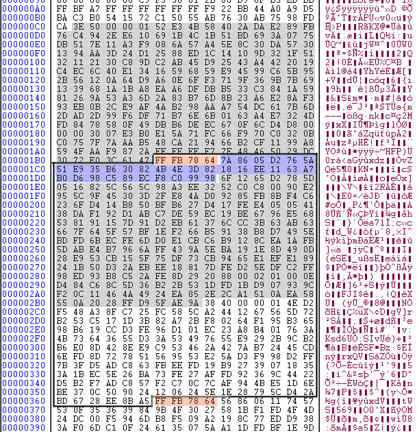
Why’s not the main data for a logical frame kept within the physical frame? At first this seems unnecessarily clumsy, but it has some advantages. The length of a physical frame is constant (within a byte) and solely based on the bit rate and other values stored in the easily found header. This makes seeking to arbitrary frames in the MP3 efficient for media players. Additionally, as frames are not limited to a fixed size in bits, parts of the audio signal with complex sounds can use bytes from preceding frames, in essence giving all MP3:s variable bit rate.
There are some limitations though: a frame can save its main data in several preceding frames, but not following frames – this would make streaming difficult. Also, the main data for a frame cannot be arbitrarily large, and is limited to about 500 bytes. This is limit is fairly short, and is often criticized.
The perceptive reader may notice the gray main data bytes in the image above begin with an interesting pattern (3E 50 00
00…) that resembles the first bytes of the main data in the next logical frame (38 40 00 00…). There is some
structure in the main data, but usually this won’t be noticeable in a hex editor.
To work with the bit stream, we are going to use a very simple type:
data MP3Bitstream = MP3Bitstream {
    bitstreamStream :: B.ByteString,
    bitstreamBuffer :: [Word8]
}
Where the ByteString is the unparsed bit stream, and the [Word8] is an internal buffer used to reconstruct
logical frames from physical frames. Not familiar with Haskell? Don’t worry; all the code in this article is only complementary.
As the bit stream may contain data we consider garbage, such as ID3 tags, we are using a simple helper function,
mp3Seek, which takes the MP3Bitstream and discards bytes until it finds a valid header. The new
MP3Bitstream can then be passed to a function that does the actual physical to logical unpacking.
mp3Seek :: MP3Bitstream -> Maybe MP3Bitstream
mp3UnpackFrame :: MP3Bitstream -> (MP3Bitstream, Maybe MP3LogicalFrame)
The anatomy of a logical frame
When we’re done decoding proper, a logical frame will have yielded us exactly 1152 time domain samples per channel. In a typical PCM WAV file, storing these samples would require 2304 bytes per channel – more than 4½ KB in total for a typical audio track. While large parts of the compression from 4½ KB audio to 0.4 KB frame stems from the removal of frequency content, a not insignificant contribution is thanks to a very efficient binary representation.
Before that, we have to make sense of the logical frame, especially the side information and the main data. When we’re done parsing the logical frame, we will have compressed audio and a bunch of parameters describing how to decompress it.
Unpacking the logical frame requires some information about the different parts. The 4-byte header stores some properties about the audio signal, most importantly the sample rate and the channel mode (mono, stereo etc). The information in the header is useful both for media player software, and for decoding the audio. Note that the header does not store many parameters used by the decoder, e.g. how audio samples should be reconstructed, those parameters are stored elsewhere.
The side information is 17 bytes for mono, 32 bytes otherwise. There’s lots of information in the side info. Most of the bits describe how the main data should be parsed, but there are also some parameters saved here used by other parts of the decoder.
The main data contains two “chunks” per channel, which are blocks of compressed audio (and corresponding parameters) decoded individually. A mono frame has two chunks, while a stereo frame has four. This partitioning is cruft left over from layer 1 and 2. Most new audio codecs designed from scratch don’t bother with this partitioning.
The first few bits of a chunk are the so-called scale factors – basically 21 numbers, which are used for decoding the chunk later. The reason the scale factors are stored in the main data and not the side information, as many other parameters, is the scale factors take up quite a lot of space. How the scale factors should be parsed, for example how long a scale factor is in bits, is described in the side information.
Following the scale factors is the actual compressed audio data for this chunk. These are a few hundred numbers, and take up most of the space in a chunk. These audio samples are actually compressed in a sense many programmers may be familiar with: Huffman coding, as used by zip, zlib and other common lossless data compression methods.
The Huffman coding is actually one of the biggest reasons an MP3 file is so small compared to the raw audio, and it’s worth investigating further. For now let’s pretend we have decoded the main data completely, including the Huffman coded data. Once we have done this for all four chunks (or two chunks for mono), we have successfully unpacked the frame. The function that does this is:
mp3ParseMainData :: MP3LogicalFrame -> Maybe MP3Data
Where MP3Data store some information, and the two/four parsed chunks.
Huffman coding
The basic idea of Huffman coding is simple. We take some data we want to compress, say a list of 8 bit characters. We then create a value table where we order the characters by frequency. If we don’t know beforehand how our list of characters will look, we can order the characters by probability of occurring in the string. We then assign code words to the value table, where we assign the short code words to the most probable values. A code word is simply an n-bit integer designed in such a way there are no ambiguities or clashes with shorter code words.
For example, lets say we have a very long string made up of the letters A, C, G and T. Being good programmers, we notice it’s wasteful to save this string as 8 bit characters, so we store them with 2 bits each. Huffman coding can compress the string further, if some of the letters are more frequent than others. In our example, we know beforehand ‘A’ occurs in the string with about 40% probability. We create a frequency table:
| A | 40% |
| C | 35% |
| G | 20% |
| T | 5% |
We then assign code words to the table. This is done in a specific way – if we pick code words at random we are not Huffman coding anymore but using a generic variable-length code.
| A | 0 |
| C | 10 |
| G | 110 |
| T | 111 |
Say we have a string of one thousand characters. If we save this string in ASCII, it will take up 8000 bits. If we instead use our 2-bit representation, it will only take 2000 bits. With Huffman coding however, we can save it in only 1850.
Decoding is the reverse of coding. If we have a bit string, say 00011111010, we read bits until there’s a match in the
table. Our example string decodes to AAATGC. Note that the code word table is designed so there are no conflicts. If the table read
| A | 0 |
| C | 01 |
… and we encounter the bit 0 in a table, there’s no way we can ever get a C as the A will match all the time.
The standard method of decoding a Huffman coded string is by walking a binary tree, created from the code word table. When we encounter a 0 bit, we move – say – left in the tree, and right when we see a 1. This is the simplest method used in our decoder.
There’s a more efficient method to decode the string, a basic time-space tradeoff that can be used when the same code word table is used to code/decode several different bit strings, as is the case with MP3. Instead of walking a tree, we use a lookup table in a clever way. This is best illustrated with an example:
lookup[0xx] = (A, 1)
lookup[10x] = (C, 2)
lookup[110] = (G, 3)
lookup[111] = (T, 3)
In the table above, xx means all permutations of 2 bits; all bit patterns from 00 to 11. Our table thus
contains all indices from 000 to 111. To decode a string using this table we peek 3 bits in the coded bit
string. Our example bit string is 00011111010, so our index is 000. This matches the pair (A, 1), which means
we have found the value A and we should discard 1 bit from the input. We peek another 3 bits in the string, and repeat the process.
For very large Huffman tables, where the longest code word is dozens of bits, it is not feasible to create a lookup table using this method of padding as it would require a table approximately 2n elements large, where n is the length of the longest code word. By carefully looking at a code word table however, it’s often possible to craft a very efficient lookup table by hand, that uses a method with “pointers” to different tables, which handle the longest code words.
How Huffman coding is used in MP3
To understand how Huffman coding is used by MP3, it is necessary to understand exactly what is being coded or decoded. The compressed data that we are about to decompress is frequency domain samples. Each logical frame has up to four chunks – two per channel – each containing up to 576 frequency samples. For a 44100 Hz audio signal, the first frequency sample (index 0) represent frequencies at around 0 Hz, while the last sample (index 575) represent a frequency around 22050 Hz.
These samples are divided into five different regions of variable length. The first three regions are known as the big values regions, the fourth region is known as the count1 region (or quad region), and the fifth is known as the zero region. The samples in the zero region are all zero, so these are not actually Huffman coded. If the big values regions and the quad region decode to 400 samples, the remaining 176 are simply padded with 0.
The three big values regions represent the important lower frequencies in the audio. The name big values refer to the information content: when we are done decoding the regions will contain integers in the range –8206 to 8206.
These three big values regions are coded with three different Huffman tables, defined in the MP3 standard. The standard defines 15 large tables for these regions, where each table outputs two frequency samples for a given code word. The tables are designed to compress the “typical” content of the frequency regions as much as possible.
To further increase compression, the 15 tables are paired with another parameter for a total of 29 different ways each of the three regions can be compressed. The side information contains information which of the 29 possibilities to use. Somewhat confusingly, the standard calls these possibilities “tables”. We will call them table pairs instead.
As an example, here is Huffman code table 1 (table1), as defined in the standard:
| Code word | Value |
|---|---|
1 | (0, 0) |
001 | (0, 1) |
01 | (1, 0) |
000 | (1, 1) |
And here is table pair 1: (table1, 0).
To decode a big values region using table pair 1, we proceed as follows: Say the chunk contains the following bits:
000101010... First we decode the bits as we usually decode Huffman coded strings: The three bits 000
correspond to the two output samples 1 and 1, we call them x and y.
Here’s where it gets interesting: The largest code table defined in the standard has samples no larger than 15. This is enough to represent most signals satisfactory, but sometimes a larger value is required. The second value in the table pair is known as the linbits (for some reason), and whenever we have found an output sample that is the maximum value (15) we read linbits number of bits, and add them to the sample. For table pair 1, the linbits is 0, and the maximum sample value is never 15, so we ignore it in this case. For some samples, linbits may be as large as 13, so the maximum value is 15+8191.
When we have read linbits for sample x, we get the sign. If x is not 0, we read one bit. This determines of the sample is positive or negative.
All in all, the two samples are decoded in these steps:
- Decode the first bits using the Huffman table. Call the samples x and y.
- If x = 15 and linbits is not 0, get linbits bits and add to x. x is now at most 8206.
- If x is not 0, get one bit. If 1, then x is –x.
- Do step 2 and 3 for y.
The count1 region codes the frequencies that are so high they have been compressed tightly, and when decoded we have samples in the range –1 to 1. There are only two possible tables for this region; these are known as the quad tables as each code word corresponds to 4 output samples. There are no linbits for the count1 region, so decoding is only a matter of using the appropriate table and get the sign bits.
- Decode the first bits using the Huffman table. Call the samples v, w, x and y.
- If v is not 0, get one bit. If 1, then v is –v.
- Do step 2 for w, x and y.
Step 1, summary
Unpacking an MP3 bit stream is very tedious, and is without doubt the decoding step that requires the most lines of code. The Huffman tables alone are a good 70 kilobytes, and all the parsing and unpacking requires a few hundred lines of code too.
The Huffman coding is undoubtedly one of the most important features of MP3 though. For a 500-byte logical frame with two channels, the output is 4x576 samples (1152 per channel) with a range of almost 15 bits, and that is even before we’ve done any transformations on the output samples. Without the Huffman coding, a logical frame would require up to 4-4½ kilobytes of storage, about an eight-fold increase in size.
All the unpacking is done by Unpack.hs, which exports two functions, mp3Seek and mp3Unpack. The latter is
a simple helper function that combines mp3UnpackFrame and mp3ParseMainData. It looks like this:
mp3Unpack :: MP3Bitstream -> (MP3Bitstream, Maybe MP3Data)
Decoding, step 2: Re-quantization
Having successfully unpacked a frame, we now have a data structure containing audio to be processed further, and parameters how this
should be done. Here are our types, what we got from mp3Unpack:
data MP3Data = MP3Data1Channels SampleRate ChannelMode (Bool, Bool)
                                MP3DataChunk MP3DataChunk
             | MP3Data2Channels SampleRate ChannelMode (Bool, Bool)
                                MP3DataChunk MP3DataChunk
                                MP3DataChunk MP3DataChunk

data MP3DataChunk = MP3DataChunk {
    chunkBlockType    :: Int,
    chunkBlockFlag    :: BlockFlag,
    chunkScaleGain    :: Double,
    chunkScaleSubGain :: (Double, Double, Double),
    chunkScaleLong    :: [Double],
    chunkScaleShort   :: [[Double]],
    chunkISParam      :: ([Int], [[Int]]),
    chunkData         :: [Int]
}
MP3Data is simply an unpacked and parsed logical frame. It contains some useful information, first is the sample rate,
second is the channel mode, third are the stereo modes (more about them later). Then are the two-four data chunks, decoded separately.
What the values stored in an MP3DataChunk represent will be described soon. For now it’s enough to know
chunkData store the (at most) 576 frequency domain samples. An MP3DataChunk is also known as a
granule, however to avoid confusion we are not going to use this term until later in the article.
Re-quantization
We have already done one of the key steps of decoding an MP3: decoding the Huffman data. We will now do the second key step – re-quantization.
As hinted in the chapter on human hearing, the heart of MP3 compression is quantization. Quantization is simply the approximation of a large range of values with a smaller set of values i.e. using fewer bits. For example if you take an analog audio signal and sample it at discrete intervals of time you get a discrete signal – a list of samples. As the analog signal is continuous, these samples will be real values. If we quantize the samples, say approximate each real valued sample with an integer between –32767 and +32767, we end up with a digital signal – discrete in both dimensions.
Quantization can be used as a form of lossy compression. For 16 bit PCM each sample in the signal can take on one of 216 values. If we instead approximate each sample in the range –16383 to +16383, we lose information but save 1 bit per sample. The difference between the original value and the quantized value is known as the quantization error, and this results in noise. The difference between a real valued sample and a 16-bit sample is so small it’s inaudible for most purposes, but if we remove too much information from the sample, the difference between the original will soon be audible.
Let’s stop for a moment and think about where this noise comes from. This requires a mathematical insight, due to Fourier: all continuous signals can be created by adding sinusoids together – even the square wave! This means that if we take a pure sine wave, say at 440 Hz, and quantize it, the quantization error will manifest itself as new frequency components in the signal. This makes sense – the quantized sine is not really a pure sine, so there must be something else in the signal. These new frequencies will be all over the spectra, and is noise. If the quantization error is small, the magnitude of the noise will be small.
And this is where we can thank evolution our ear is not perfect: If there’s a strong signal within a critical band, the noise due to quantization errors will be masked, up to the threshold. The encoder can thus throw away as much information as possible from the samples within the critical band, up to the point were discarding more information would result in noise passing the audible threshold. This is the key insight of lossy audio encoding.
Quantization methods can be written as mathematical expressions. Say we have a real valued sample in the range –1 to 1. To quantize
this value to a form suitable for a 16 bit WAV file, we multiply the sample with 32727 and throw away the fractional part: q = floor(s
* 32767) or equivalently in a form many programmers are familiar with: (short)(s * 32767.0). Re-quantization in this
simple case is a division, where the difference between the re-quantized sample and the original is the quantization error.
Re-quantization in MP3
After we unpacked the MP3 bit stream and Huffman decoded the frequency samples in a chunk, we ended up with quantized frequency samples between –8206 and 8206. Now it’s time to re-quantize these samples to real values (floats), like when we take a 16-bit PCM sample and turn it to a float. When we’re done we have a sample in the range –1 to 1, much smaller than 8206. However our new sample has a much higher resolution, thanks to the information the encoder left in the frame how the sample should be reconstructed.
The MP3 encoder uses a non-linear quantizer, meaning the difference between consecutive re-quantized values is not constant. This is because low amplitude signals are more sensitive to noise, and thus require more bits than stronger signals – think of it as using more bits for small values, and fewer bits for large values. To achieve this non-linearity, the different scaling quantities are non-linear.
The encoder will first raise all samples by 3/4, that is newsample = oldsample3/4. The purpose is, according to the literature, to make the signal-to-noise ratio more consistent. We will gloss over the why’s and how’s here, and just raise all samples by 4/3 to restore the samples to their original value.
All 576 samples are then scaled by a quantity simply known as the gain, or the global gain because all samples are affected. This is
chunkScaleGain, and it’s also a non-linear value.
This far, we haven’t done anything really unusual. We have taken a value, at most 8206, and scaled it with a variable quantity. This is not that much different from a 16 bit PCM WAV, where we take a value, at most 32767, and scale it with the fixed quantity 1/32767. Now things will get more interesting.
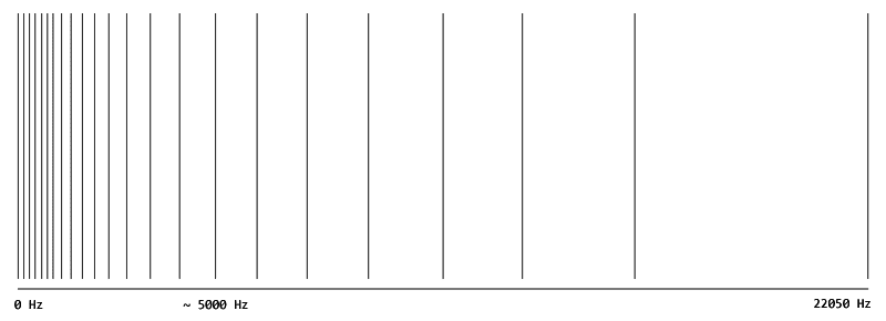
Some frequency regions, partitioned into several scale factor bands, are further scaled individually. This is what the scale factors are for: the frequencies in the first scale factor band are all multiplied by the first scale factor, etc. The bands are designed to approximate the critical bands. Here’s an illustration of the scale factor bandwidths for a 44100 Hz MP3. The astute reader may notice there are 22 bands, but only 21 scale factors. This is a design limitation that affects the very high frequencies.
The reason these bands are scaled individually is to better control quantization noise. If there’s a strong signal in one band, it will mask the noise in this band but not others. The values within a scale factor band are thus quantized independently from other bands by the encoder, depending on the masking effects.
Because of reasons that will hopefully be made more clear shortly, a chunk can be scaled in three different ways.
For one type of chunk – called “long” – we scale the 576 frequencies by the global gain and the 21 scale factors
(chunkScaleLong), and leave it at that.
For another type of chunk – called “short” – the 576 samples are really three interleaved sets of 192 frequency samples. Don’t worry
if this doesn’t make any sense now, we will talk about it soon. In this case, the scale factor bands look slightly different than in
the illustration above, to accommodate the reduced bandwidths of the scale factor bands. Also, the scale factors are not 21 numbers,
but sets of three numbers (chunkScaleShort). An additional parameter, chunkScaleSubGain, further scales the
individual three sets of samples.
The third type of chunk is a mix of the above two.
When we have multiplied each sample with the corresponding scale factor and other gains, we are left with a high precision floating point representation of the frequency domain, where each sample is in the range –1 to 1.
Here’s some code, that uses almost all values in a MP3DataChunk. The three different scaling methods are controlled by
the BlockFlag. There will be plenty more information about the block flag later in this article.
mp3Requantize :: SampleRate -> MP3DataChunk -> [Frequency]
mp3Requantize samplerate (MP3DataChunk bt bf gain (sg0, sg1, sg2)
                         longsf shortsf _ compressed)
    | bf == LongBlocks  = long
    | bf == ShortBlocks = short
    | bf == MixedBlocks = take 36 long ++ drop 36 short
    where
        long  = zipWith procLong  compressed longbands
        short = zipWith procShort compressed shortbands

        procLong sample sfb =
            let localgain   = longsf !! sfb
                dsample     = fromIntegral sample
            in gain * localgain * dsample **^ (4/3)

        procShort sample (sfb, win) =
            let localgain = (shortsf !! sfb) !! win
                blockgain = case win of 0 -> sg0
                                        1 -> sg1
                                        2 -> sg2
                dsample   = fromIntegral sample
            in gain * localgain * blockgain * dsample **^ (4/3)

        -- Frequency index (0-575) to scale factor band index (0-21).
        longbands = tableScaleBandIndexLong samplerate
        -- Frequency index to scale factor band index and window index (0-2).
        shortbands = tableScaleBandIndexShort samplerate
A fair warning: This presentation of the MP3 re-quantization step differs somewhat from the official specification. The specification presents the quantization as a long formula based on integer quantities. This decoder instead treats these integer quantities as floating point representations of non-linear quantities, so the re-quantization can be expressed as an intuitive series of multiplications. The end result is the same, but the intention is hopefully clearer.
Minor step: Reordering
Before quantizing the frequency samples, the encoder will in certain cases reorder the samples in a predefined way. We have already encountered this above: after the reordering by the encoder the “short” chunks with three small chunks of 192 samples each are combined to 576 samples ordered by frequency (sort of). This is to improve the efficiency of the Huffman coding, as the method with big values and different tables assume the lower frequencies are first in the list.
When we’re done re-quantizing in our decoder, we will reorder the “short” samples back to their original position. After this reordering, the samples in these chunks are no longer ordered by frequency. This is slightly confusing, so unless you are really interested in MP3 you can ignore this and concentrate on the “long” chunks, which have very few surprises.
Decoding, step 3: Joint Stereo
MP3 supports four different channel modes. Mono means the audio has a single channel. Stereo means the audio has two channels. Dual channel is identical to stereo for decoding purposes – it’s intended as information for the media player in case the two channels contain different audio, such as an audio book in two languages.
Then there’s joint stereo. This is like the regular stereo mode, but with some extra compression steps taking similarities between the two channels into account. This makes sense, especially for stereo music where there’s usually a very high correlation between the two channels. By removing some redundancy, the audio quality can be much higher for a given bit rate.
MP3 supports two joint stereo modes known as middle/side stereo (MS) and intensity stereo (IS). Whether these modes
are in use is given by the (Bool, Bool) tuple in the MP3Data type. Additionally chunkISParam
stores parameter used by IS mode.
MS stereo is very simple: instead of encoding two similar channels verbatim, the encoder computes the sum and the difference of the two channels before encoding. The information content in the “side” channel (difference) will be less than the “middle” channel (sum), and the encoder can use more bits for the middle channel for a better result. MS stereo is lossless, and is a very common mode that’s often used in joint stereo MP3:s. Decoding MS stereo is very cute:
mp3StereoMS :: [Frequency] -> [Frequency] -> ([Frequency], [Frequency])
mp3StereoMS middle side =
    let sqrtinv = 1 / (sqrt 2)
        left  = zipWith0 (\x y -> (x+y)*sqrtinv) 0.0 middle side
        right = zipWith0 (\x y -> (x-y)*sqrtinv) 0.0 middle side
    in (left, right)
The only oddity here is the division by the square root of 2 instead of simply 2. This is to scale down the channels for more efficient quantization by the encoder.
A more unusual stereo mode is known as intensity stereo, or IS for short. We will ignore IS stereo in this article.
Having done the stereo decoding, the only thing remaining is taking the frequency samples back to the time domain. This is the part heavy on theory.
Decoding, step 4: Frequency to time
At this point the only remaining MP3DataChunk values we will use are chunkBlockFlag and
chunkBlockType. These are the sole two parameters that dictate how we’re going to transform our frequency domain samples
to the time domain. To understand the block flag and block type we have to familiarize ourselves with some transforms, as well as one
part of the encoder.
The encoder: filter banks and transforms
The input to an encoder is probably a time domain PCM WAV file, as one usually gets when ripping an audio CD. The encoder takes 576
time samples, from here on called a granule, and encodes two of these granules to a frame. For an input source with two channels, two
granules per channel are stored in the frame. The encoder also saves information how the audio was compressed in the frame. This is the
MP3Data type in our decoder.
The time domain samples are transformed to the frequency domain in several steps, one granule a time.
Analysis filter bank
First the 576 samples are fed to a set of 32 band pass filters, where each band pass filter outputs 18 time domain samples representing 1/32:th of the frequency spectra of the input signal. If the sample rate is 44100 Hz each band will be approximately 689 Hz wide (22050/32 Hz). Note that there’s downsampling going on here: Common band pass filters will output 576 output samples for 576 input samples, however the MP3 filters also reduce the number of samples by 32, so the combined output of all 32 filters is the same as the number of inputs.
This part of the encoder is known as the analysis filter bank (throw in the word polyphase for good measure), and it’s a part of the encoder common to all the MPEG-1 layers. Our decoder will do the reverse at the very end of the decoding process, combining the subbands to the original signal. The reverse is known as the synthesis filter bank. These two filter banks are simple conceptually, but real mammoths mathematically – at least the synthesis filter bank. We will treat them as black boxes.
MDCT
The output of each band pass filter is further transformed by the MDCT, the modified discrete cosine transform. This transform is just a method of transforming the time domain samples to the frequency domain. Layer 1 and 2 does not use this MDCT, but it was added on top of the filter bank for layer 3 as a finer frequency resolution than 689 Hz (given 44.1 KHz sample rate) proved to give better compression. This makes sense: simply dividing the whole frequency spectra in fixed size blocks means the decoder has to take several critical bands into account when quantizing the signal, which results in a worse compression ratio.
The MDCT takes a signal and represents it as a sum of cosine waves, turning it to the frequency domain. Compared to the DFT/FFT and other well-known transforms, the MDCT has a few properties that make it very suited for audio compression.
First of all, the MDCT has the energy compaction property common to several of the other discrete cosine transforms. This means most of the information in the signal is concentrated to a few output samples with high energy. If you take an input sequence, do an (M)DCT transform on it, set the “small” output values to 0, then do the inverse transform – the result is a fairly small change in the original input. This property is of course very useful for compression, and thus different cosine transforms are used by not only MP3 and audio compression in general but also JPEG and video coding techniques.
Secondly, the MDCT is designed to be performed on consecutive blocks of data, so it has smaller discrepancies at block boundaries compared to other transforms. This also makes it very suited for audio, as we’re almost always working with really long signals.
Technically, the MDCT is a so-called lapped transform, which means we use input samples from the previous input data when we work with the current input data. The input is 2N time samples and the output is N frequency samples. Instead of transforming 2N length blocks separately, consecutive blocks are overlapped. This overlapping helps reducing artifacts at block boundaries. First we perform the MDCT on say samples 0-35 (inclusive), then 18-53, then 36-71… To smoothen the boundaries between consecutive blocks, the MDCT is usually combined with a windowing function that is performed prior to the transform. A windowing function is simply a sequence of values that are zero outside some region, and often between 0 and 1 within the region, that are to be multiplied with another sequence. For the MDCT smooth, arc-like window functions are usually used, which makes the boundaries of the input block go smoothly to zero at the edges.
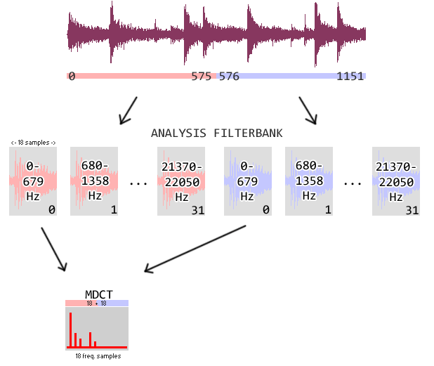
In the case of MP3, the MDCT is done on the subbands from the analysis filter bank. In order to get all the nice properties of the
MDCT, the transform is not done on the 18 samples directly, but on a windowed signal formed by the concatenation of the 18 previous and
the current samples. This is illustrated in the picture below, showing two consecutive granules (MP3DataChunk) in an audio
channel. Remember: we are looking at the encoder here, the decoder works in reverse. This illustration shows the MDCT of the 0-679 Hz
band.
The MDCT can either be applied to the 36 samples as described above, or three MDCT:s are done on 12 samples each – in either case the output is 18 frequency samples. The first choice, known as the long method, gives us greater frequency resolution. The second choice, known as the short method, gives us greater time resolution. The encoder selects the long MDCT to get better audio quality when the signal changes very little, and it selects short when there’s lots going on, that is for transients.
For the whole granule of 576 samples, the encoder can either do the long MDCT on all 32 subbands – this is the long block mode, or it can do the short MDCT in all subbands – this is the short block mode. There’s a third choice, known as the mixed block mode. In this case the encoder uses the long MDCT on the first two subbands, and the short MDCT on the remaining. The mixed block mode is a compromise: it’s used when time resolution is necessary, but using the short block mode would result in artifacts. The lowest frequencies are thus treated as long blocks, where the ear is most sensitive to frequency inaccuracies. Notice that the boundaries of the mixed block mode is fixed: the first two, and only two, subbands use the long MDCT. This is considered a design limitation of MP3: sometimes it’d be useful to have high frequency resolution in more than two subbands. In practice, many encoders do not support mixed blocks.
We discussed the block modes briefly in the chapter on re-quantization and reordering, and hopefully that part will make a little more sense knowing what’s going on inside the encoder. The 576 samples in a short granule are really 3x 192 small granules, but stored in such a way the facilities for compressing a long granule can be used.
The combination of the analysis filter bank and the MDCT is known as the hybrid filter bank, and it’s a very confusing part of the decoder. The analysis filter bank is used by all MPEG-1 layers, but as the frequency bands does not reflect the critical bands, layer 3 added the MDCT on top of the analysis filter bank. One of the features of AAC is a simpler method to transform the time domain samples to the frequency domain, which only use the MDCT, not bothering with the band pass filters.
The decoder
Digesting this information about the encoder leads to a startling realization: we can’t actually decode granules, or frames, independently! Due to the overlapping nature of the MDCT we need the inverse-MDCT output of the previous granule to decode the current granule.
This is where chunkBlockType and chunkBlockFlag are used. If chunkBlockFlag is set to the
value LongBlocks, the encoder used a single 36-point MDCT for all 32 subbands (from the filter bank), with overlapping
from the previous granule. If the value is ShortBlocks instead, three shorter 12-point MDCT:s were used.
chunkBlockFlag can also be MixedBlocks. In this case the two lower frequency subbands from the filter bank
are treated as LongBlocks, and the rest as ShortBlocks.
The value chunkBlockType is an integer, either 0,1,2 or 3. This decides which window is used. These window functions
are pretty straightforward and similar, one is for the long blocks, one is for the three short blocks, and the two others are used
exactly before and after a transition between a long and short block.
Before we do the inverse MDCT, we have to take some deficiencies of the encoder’s analysis filter bank into account. The downsampling in the filter bank introduces some aliasing (where signals are indistinguishable from other signals), but in such a way the synthesis filter bank cancels the aliasing. After the MDCT, the encoder will remove some of this aliasing. This, of course, means we have to undo this alias reduction in our decoder, prior the IMDCT. Otherwise the alias cancellation property of the synthesis filter bank will not work.
When we’ve dealt with the aliasing, we can IMDCT and then window, remembering to overlap with the output from the previous granule. For short blocks, the three small individual IMDCT inputs are overlapped directly, and this result is then treated as a long block.
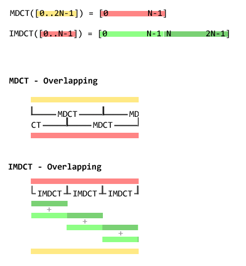
The word “overlap” requires some clarifications in the context of the inverse transform. When we speak of the MDCT, a function from 2N inputs to N outputs, this just means we use half the previous samples as inputs to the function. If we’ve just MDCT:ed 36 input samples from offset 0 in a long sequence, we then MDCT 36 new samples from offset 18.
When we speak of the IMDCT, a function from N inputs to 2N outputs, there’s an addition step needed to reconstruct the original sequence. We do the IMDCT on the first 18 samples from the output sequence above. This gives us 36 samples. Output 18..35 are added, element wise, to output 0..17 of the IMDCT output of the next 18 samples. Here’s an illustration.
With that out of the way, here’s some code:
mp3IMDCT :: BlockFlag -> Int -> [Frequency] -> [Sample] -> ([Sample], [Sample])
mp3IMDCT blockflag blocktype freq overlap =
    let (samples, overlap') =
            case blockflag of
                 LongBlocks  -> transf (doImdctLong blocktype) freq
                 ShortBlocks -> transf (doImdctShort) freq
                 MixedBlocks -> transf (doImdctLong 0)  (take 36 freq) <++>
                                transf (doImdctShort) (drop 36 freq)
        samples' = zipWith (+) samples overlap
    in (samples', overlap')
    where
        transf imdctfunc input = unzipConcat $ mapBlock 18 toSO input
            where
                -- toSO takes 18 input samples b and computes 36 time samples
                -- by the IMDCT. These are further divided into two equal
                -- parts (S, O) where S are time samples for this frame
                -- and O are values to be overlapped in the next frame.
                toSO b = splitAt 18 (imdctfunc b)
                unzipConcat xs = let (a, b) = unzip xs
                                 in (concat a, concat b)

doImdctLong :: Int -> [Frequency] -> [Sample]
doImdctLong blocktype f = imdct 18 f `windowWith` tableImdctWindow blocktype

doImdctShort :: [Frequency] -> [Sample]
doImdctShort f = overlap3 shorta shortb shortc
  where
    (f1, f2, f3) = splitAt2 6 f
    shorta       = imdct 6 f1 `windowWith` tableImdctWindow 2
    shortb       = imdct 6 f2 `windowWith` tableImdctWindow 2
    shortc       = imdct 6 f3 `windowWith` tableImdctWindow 2
    overlap3 a b c =
      p1 ++ (zipWith3 add3 (a ++ p2) (p1 ++ b ++ p1) (p2 ++ c)) ++ p1
      where
        add3 x y z = x+y+z
        p1         = [0,0,0, 0,0,0]
        p2         = [0,0,0, 0,0,0, 0,0,0, 0,0,0]
Before we pass the time domain signal to the synthesis filter bank, there’s one final step. Some subbands from the analysis filter bank have inverted frequency spectra, which the encoder corrects. We have to undo this, as with the alias reduction.
Here are the steps required for taking our frequency samples back to time:
- [Frequency] Undo the alias reduction, taking the block flag into account.
- [Frequency] Perform the IMDCT, taking the block flag into account.
- [Time] Invert the frequency spectra for some bands.
- [Time] Synthesis filter bank.
A typical MP3 decoder will spend most of its time in the synthesis filter bank – it is by far the most computationally heavy part of the decoder. In our decoder, we will use the (slow) implementation from the specification. Typical real world decoders, such as the one in your favorite media player, use a highly optimized version of the filter bank using a transform in a clever way. We will not delve in this optimization technique further.
Step 4, summary
It’s easy to miss the forest for the trees, but we have to remember this decoding step is conceptually simple; it’s just messy in MP3 because the designers reused parts from layer 1, which makes the boundaries between time domain, frequency domain and granule less clear.
Using the decoder
Using the decoder is a matter of creating a bit stream, initializing it (mp3Seek), unpacking it to an
MP3Data (mp3Unpack) and then decoding the MP3Data with mp3Decode. The decoder does
not use any advanced Haskell concepts externally, such as state monads, so hopefully the language will not get in the way of the
audio.
module Codec.Audio.MP3.Decoder (
    mp3Seek
   ,mp3Unpack
   ,MP3Bitstream(..)
   ,mp3Decode
   ,MP3DecodeState(..)
   ,emptyMP3DecodeState
) where
...

mp3Decode :: MP3DecodeState -> MP3Data -> (MP3DecodeState, [Sample], [Sample])

data MP3DecodeState = ...

emptyMP3DecodeState :: MP3DecodeState
emptyMP3DecodeState = ...
The code is tested with a new version of GHC. The decoder requires binary-strict, which can be found at Hackage. See README in the code for build
instructions. Please note that the software is currently version 0.0.1 – it’s very, very slow, and has some missing features.
Code: mp3decoder-0.0.1.tar.gz.
Conclusion
MP3 has its peculiarities, especially the hybrid filter bank, but it’s still a nice codec with a firm grounding in psychoacoustic principles. Not standardizing the encoder was a good choice by the MPEG-1 team, and the available encoders show it’s possible to compress audio satisfactory within the constraints set by the decoder.
If you decide to play around with the source code, be sure to set your sound card to a low volume if you use headphones! Removing parts of the decoder may result in noise. Have fun.
References
CD 11172-3 Part 3 (the specification)
David Salomon, Data Compression: The Complete Reference, 3rd ed.
Davis Pan, A Tutorial on MPEG/Audio Compression
Rassol Raissi, The Theory Behind Mp3
The source code to libmad, LAME and 8Hz-mp3.
posted by Björn Edström at
Wednesday, October 01, 2008
![]()

<< Home